Adaptive optimization algorithm for ultrasonic localization of transformer partial discharge
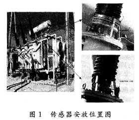
| The ultrasonic positioning method of transformer partial discharge source is accomplished by using ultrasonic emission, propagation and measurement technology. During the long-term operation of power transformer, when partial discharge occurs in some weak parts of internal insulation under the action of high field strength [1], ultrasonic energy is emitted, spherical ultrasound is propagated outward in different media, transducers at different points around the transformer can receive ultrasonic signal, which is transmitted to the background through GPRS network, and the time delay of ultrasonic signal propagation is measured in the background. The location of partial discharge points can be obtained by solving the positioning equations together. 1 Mathematical model for ultrasonic localization of partial discharge in transformer Set the partial discharge point in power transformer as S (x, y, z), x, y, Z are unknown quantities. There are eight sensors mounted on the transformer surface to receive ultrasound signals, as shown in Figure 1.
Their coordinates are Ri (xi, yi, zi), where I = 1, 2,..., 8; When the sensor receives the ultrasound signal, it returns to the background program, calculates the time difference between one of the ultrasound signals and the rest of the signals according to the correlation function method, and represents the time delay between the first (i=2, 3,..., 8) receiving end and the first receiving end with Delta ti1=ti-t1, as shown in Figure 2. υ Represents the speed of ultrasonic propagation, which is unknown due to the complex internal structure of the transformer[1].
1.1 Modeling Ideally, eight sensors can receive ultrasound signals and calculate time delays, then the equation group of the localization algorithm is:
In fact, since there are usually less than eight receivers of the signal due to the diffraction, transmission, reflection and attenuation of the ultrasound in the course of propagation, it may be advisable to assume that m+1 receivers receive the signal in the actual acquisition process. There are m non-linear positioning equations:
L.2 unconstrained optimization The positioning equation has four unknown quantities (x, y, z, υ), When 4< When m < 7, the overdetermined equations are nonlinear and have no solution. Converts an overdetermined system of equations to an unconstrained problem with the objective function of: 2 Algorithmic Description There are many classical algorithms to solve unconstrained optimization problems. The steepest descent method has simple structure, small computational effort and global convergence, but it is prone to oscillation (orthogonal) near the extreme point [4]. Newton's method converges fast, but not globally. For this reason, an adaptive algorithm [6] is presented, which shows its superiority over Newton method and the steepest descent method in transformer partial discharge location. 2.1 Algorithmic steps (1) Given the initial point X0 < R4, ε& Lt; 10-6, k=0; (2) Calculate F(Xk) to test whether the criteria for convergence are satisfied: F(Xk)= 0 ε, If it is satisfied, the iteration stops and the resulting point X*Xk is the extreme point. Otherwise (3); (3) Make Sk=-F(Xk), start from Xk, search along Sk in one dimension, that is, demand λ K, so that: (4) Order XK+1=XK+ λKSK, k=k+1; (5) To determine whether the k+1 and K gradient vectors are orthogonal or nearly orthogonal, that is, whether the orthogonal conditions are satisfied: F(Xk)? _F (Xk+1) = 0.1, if there is no orthogonality (i.e. oscillation), proceed (2); Otherwise (6); (6) Perform Newton iteration to calculate F(Xk) if F(Xk)is less than or equal to ε Stop, output Xk; Otherwise, proceed (7); (7) Calculate Sk=-[2F(Xk)]-1*gk; (8) One-dimensional search: min F (Xk+ λ Sk) = F (Xk+ λ KSk), so Xk+1 = Xk+ λ KSk, k = K + 1, proceed (6). In the algorithm, to select an appropriate initial point for the unknown vector before starting iteration, the selection of the initial point is often related to the success of the algorithm. Consider a method that divides a transformer into volumetric elements of the same size. The number of volumetric elements can be tens or even hundreds. Each element's geometric center is used as the initial point to iterate successively. After the iteration, the points in the entire transformer are determined by comparing the iteration results of all the elements. 2.3 Algorithmic Analysis This algorithm combines the steepest descent method with Newton method, selects the initial point based on the voxel division, and begins the iteration. With the global convergence of the steepest descent method, the initial optimization process is completed before the oscillation of the gradient vector occurs, and then the Newton method is used to optimize the gradient vector. The Newton method has a fast convergence speed and the iteration results can meet the requirements within 10 steps. Application of 3 Combination Algorithms in Partial Discharge Point Location of Power Transformer In the project of transformer partial discharge on-line detection in Shanxi Yuncheng Power Supply Company, the algorithm is applied. The following is the on-site detection. Site 1 inspection: Transformer Rule (Long) × wide × High):1.2 M × 0.8 m × 1.0 m; Actual discharge point coordinates: S (0.5, 0.4, 0.4); Sensor coordinates: R1 (0.6, 0.0, 0.5), R2 (0.0, 0.4, 0.5), R3 (0.6, 0.4, 1.0), R4 (1.2, 0.4, 0.5), R5 (0.6, 0.8, 0.5); Reference point time: t1=0.000 303 05 s; Receive delay: d1=[0.000 364 22; 0.000 434 48; 0.000 505 08; 0.000 1286] one t1. Number of voids: 5 × 5 × 5.
Site 2 inspection: Transformer Rule (Long) × wide × High):5 M × 3 M × 4 m; Actual discharge point coordinates: S (4.5, 2.6, 3.7); Receiver coordinates: R1 (2.5, 0.0, 2.0), R2 (2.5, 1.5, 4.0), R3 (5.0, 1.5, 2.O), R4 (2.5, 3.0, 2.0), R5 (0, 1.5, 2.0); Reference point time: t1=0.002 6S; Receive delay: d1=[0.001 6; 0.001 5; 0.001 9; 0.003 524 69] one t1. Number of voids: 5 × 5 × 5.
4 Conclusion Field detection reflects the superiority of hybrid algorithm, mainly: (1) The combination algorithm has the advantage of global convergence of the steepest descent method; (2) The combination algorithm has the advantage of fast convergence of Newton method; (3) The initial points are divided automatically and discriminated automatically to ensure the global situation; (4) 10 cm with different data, which completely meets the requirements of discharge positioning. | |||||||||


Source:Xiang Xueqin
Copyright & Disclaimer
All works on this website that state "Source: ICMoment", all copyright belongs to ICMoment, please
specify
icmoment, https://www.icmoment.com, violators will be investigated for related The website will be held
legally responsible.
This website reproduces and indicates works from other sources, the purpose is to pass on more
information,
does not mean that the network agrees with its views or to confirm the authenticity of its content, does
not
assume direct responsibility for such works of infringement and joint and several liability. When other
media, websites or individuals reprint from this website, they must retain the source of the work
indicated
on this website and bear their own legal responsibility for copyright and other issues.
If the content of the work, copyright and other issues are involved, please contact us within one week from the date of publication of the work, otherwise it is regarded as a waiver of the relevant rights.
Related Readings
Popular Circuit Diagrams
Special Sale
Model
Price
